21 Deep Learning

Deep learning is a subset of machine learning that uses neural networks to learn from data. The aim of neural networks is to mimic the human brain.

Perceptron Model to Neural Networks

Perceptron Model

A perceptron was a form of neural network introduced in 1958 by Frank Rosenblatt.
The human brain is made up of billions of neurons that are connected to each other. Each neuron is connected to other neurons through synapses. The synapses are
responsible for transmitting information from one neuron to another.
the following image represent a simplified model of a neuron that takes inputs and produces an output.
What's biologically called "dentrites" are the inputs of the neuron, the "nucleus" is the processing unit and the "axon" is the output of the neuron.

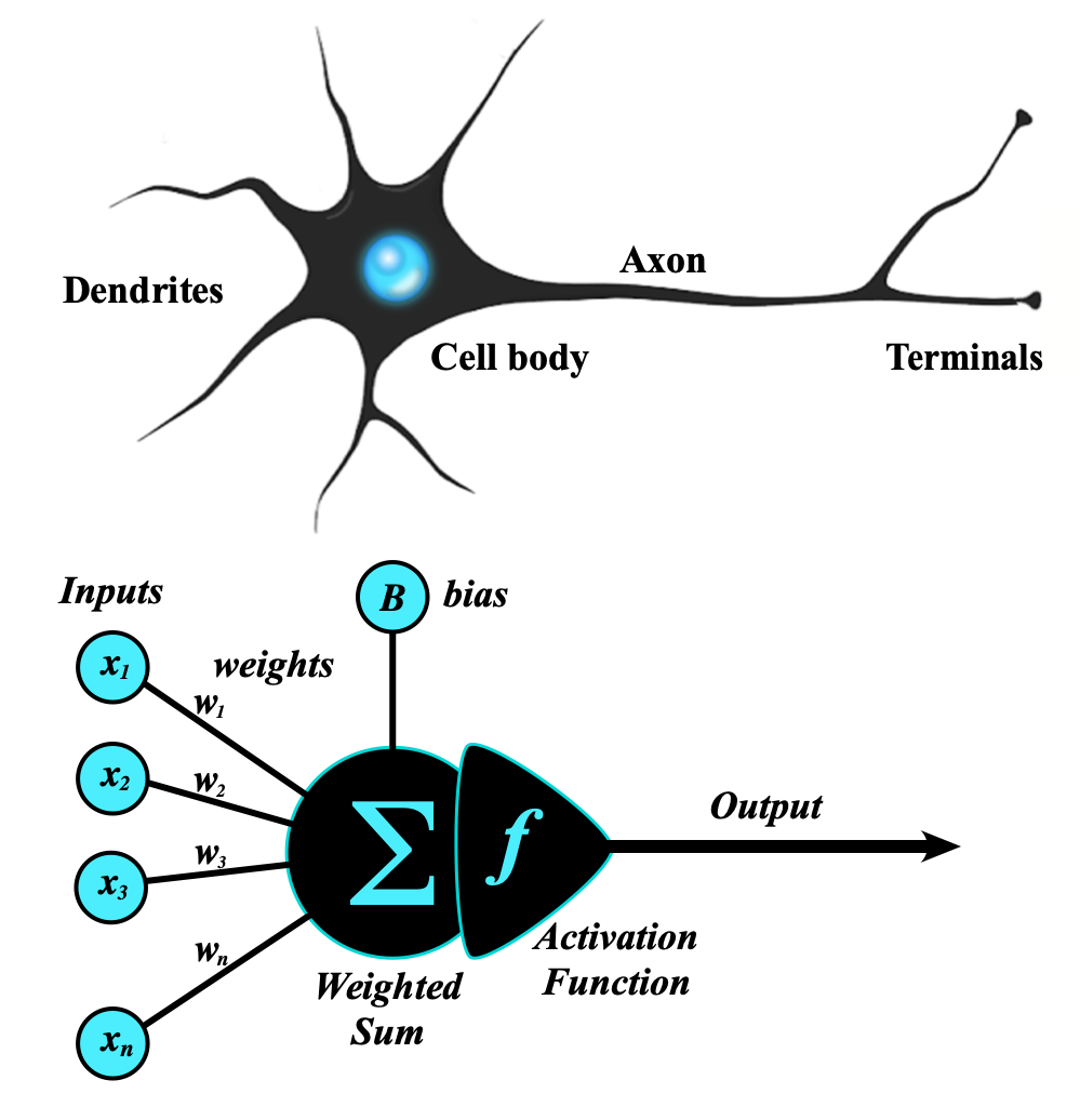
The mathemtical representation highlights the similarity with the biological model where the neuron takes inputs and produces an output. It's possible to imagine that inside the nucleus there is a function that takes the inputs and produces an output.

Ex. if F(x) is a sum the perceptron model will be: y=x1+x2

Is used to multiply the inputs by a weight and then sum them up. The weights are the parameters of the model and they are used to learn from the data. It's useful to think of the weights as the strength of the synapses in the biological model.

The equation becomes: y=w1x1+w2x2

There's still a prolem, if the input X is 0 the output will always be 0. To solve this problem is used a bias that is added to the equation. The bias is a constant value that ensures that the output is not always 0.

The equation becomes: y=(x1w1 + b) + (x2w2 + b)

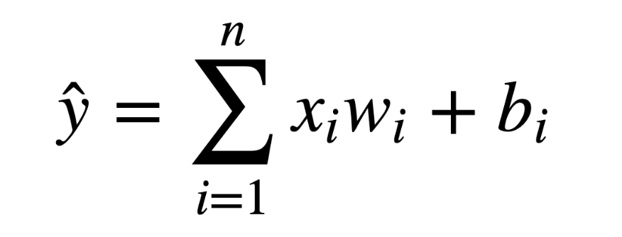
The mathematical generalization of the perceptron model is:

Neural Networks

A neural network is a collection of perceptrons that are connected to each other.
A multi-layer perceptron model is known as basic artificial neural network.
The following image represents a neural network with 3 inputs, 2 hidden layers and 1 output.

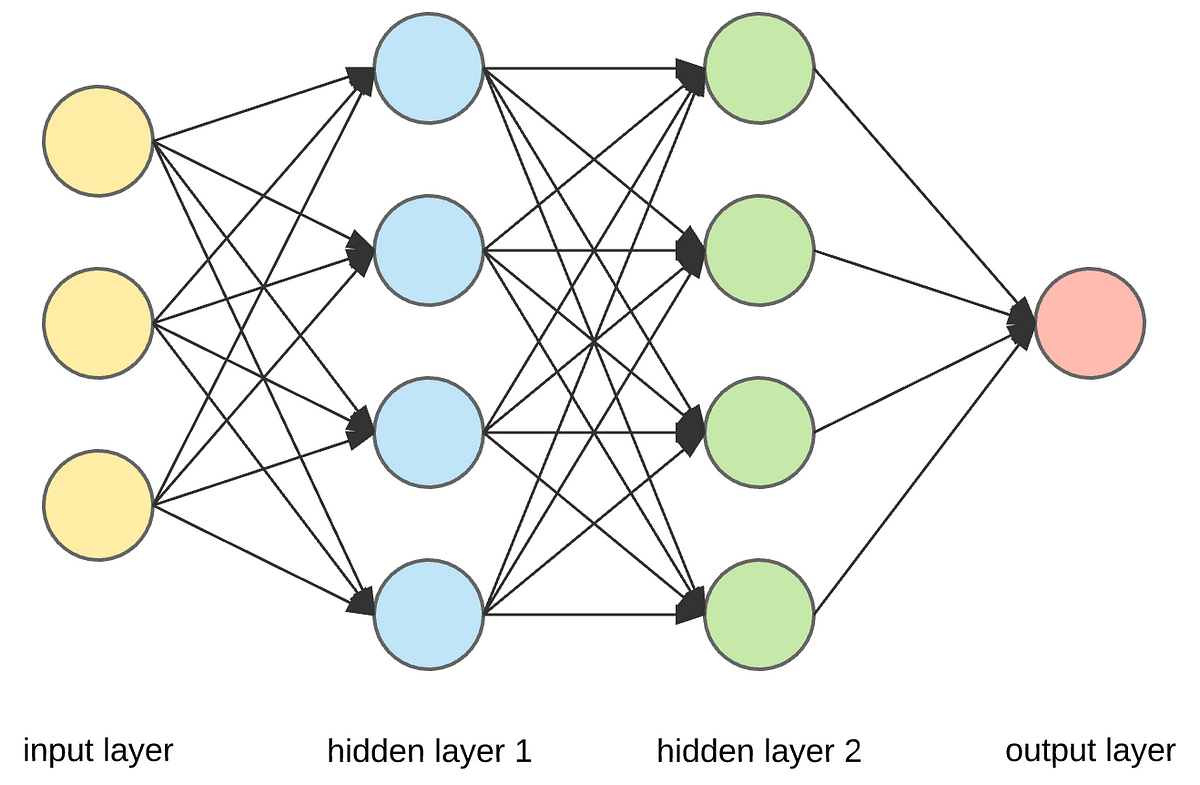
The output of the previous layer is the input of the next layer. The first layer is called input layer, the last layer is called output layer and the layers in between are called hidden layers.
A fully connected layer is a layer in which each neuron is connected to every neuron in the previous layer.
In case of multiclass classification the output layer will have as many neurons as the number of classes. The output of each neuron will be the probability of the input to belong to that class.

Hidden layers are difficoult to interpret and understand because of their high interconnectivity. The weights of the hidden layers are not directly related to the input and output. The hidden layers are used to learn the features of the data.

• Neural networks become "deep neural networks" when they have more than one hidden layer.
• The width of a network is the number of neurons in a layer.
• The depth of a network is the number of layers in the network.

The incredible thing about the neural network framework is that it can be used to appoximate any function. This is known as the universal approximation theorem.
Has been proven that a neural network with a single hidden layer can approximate any function. The number of neurons in the hidden layer is the only thing that changes.

Activation Functions

Considering the formula x*w + b where a weight and a bias are applied to entry x variable it's possible to say that w is the strength applied to x and the bias is the offset applied to x in order to reach a certain threshold.
It's possible to say that the bias is assigned based on the weight of the input. If the weight is high the bias will be low and viceversa.

Ex. if b=-10 and w=0.5 the threshold will be 20. If b=-10 and w=2 the threshold will be 5.

For activation function is meant a function that is applied to the output of a neuron. The activation function is used to introduce non-linearity in the model.
Changing the activation function means changing the shape of the output of the neuron.

Sigmoid Function

The sigmoid function is a function that takes a real value as input and outputs another value between 0 and 1. The sigmoid function is used to convert a real value to a probability value.
Considering a binary classification problem the output of the sigmoid function can be used to predict the probability of the input to belong to a certain class.
By returning a number between 0 an 1 it provides a probability that the input belongs to a certain class.

Sigmoid function has been used as activation function in the past but it's not used anymore because it has some problems:

• The gradient of the sigmoid function is very small for very high and very low values. This means that the gradient descent will be very slow.
• The output of the sigmoid function is not zero centered. This means that the gradient descent will be zig-zagging and it will be slower.
• The output of the sigmoid function is not sparse. This means that the output will be always between 0 and 1.
• The sigmoid function is computationally expensive.
• The sigmoid function doesn't punish outliers.

The sigmoid function is also known as logistic function and is defined as:

f(z) = 1 / (1 + e^(-z))

Hyperbolic Tangent Function

The hyperbolic tangent function is a really common option and takes a real value as input and outputs another value between -1 and 1. The hyperbolic tangent function is used to convert a real value to a probability value.
Also existing the hyperbolin sin and the hyperbolic cosine functions but if preferred the hyperbolic tangent function because it's zero centered.
The hyperbolic tangent function is defined as:

f(z) = (e^z - e^(-z)) / (e^z + e^(-z))

Rectified Linear Unit Function

The rectified linear unit function is a function that takes a real value as input and outputs another value between 0 and infinity. The rectified linear unit function is used to convert a real value to a probability value.

It considers values smaller than 0 as 0 and values greater than 0 as they are.

It has a lot of advantages:

• It as good performance while dealing with the issue of vanishing gradient: the gradient is not zero for positive values.
• It's computationally efficient.
• It's sparse: the output is zero for negative values.

The rectified linear unit function is defined as:

f(z) = max(0, z)

Cost Functions

Cost functions are functions that measure the performance of a model for given data. The cost function is used to estimate the parameters of the model.

Const functions deals with N-dimensional vectors (tensors) that instead of using derivatives use gradients.
The gradient is calculated in the following way:

C(w) = (Delta<C(w1), C(w2), ..., C(wn)>)

Learning Rate

The learning rate is a hyperparameter that controls how much to change the model in response to the estimated error each time the model weights are updated.
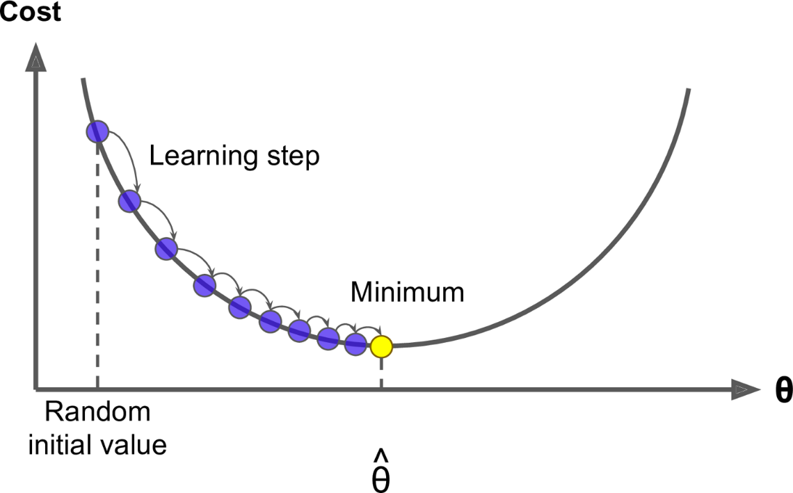
The following plot represents the error of the model as a function of the learning rate. The learning rate is the x-axis and the error is the y-axis.
The minimum value of the error is the optimal learning rate. If the learning rate is too small the model will take a lot of time to converge. If the learning rate is too big the model will never converge.
It's also possible to use an adaptive gradient descent that changes the learning rate during the training process.

Adam Optimizer

Adam is an optimization algorithm published in 2015 that can be used instead of the classical stochastic gradient descent procedure to update network weights iterative based in training data.
Adam is a much more efficient version of the gradient descent algorithm. Adam is an adaptive learning rate optimization algorithm that's been designed specifically for training deep neural networks.

Quadratic Cost Function

The quadratic cost function is a very common function that takes the difference between the predicted value and the actual value and squares it. The quadratic cost function is used to measure the performance of a regression model.
pros:

• keeps everything positive
• punishes outliers
  cons:
• The quadratic cost function is not used for classification problems.

Cross Entropy Cost Function

The cross entropy cost function is a very common function that takes the difference between the predicted value and the actual value and squares it. The cross entropy cost function is used to measure the performance of a classification model.

Feed Forward Neural Networks

Backpropagation

Backpropagation is an algorithm used to train neural networks, it gets back to the output of the network and propagates the error backward through the network in order to update the weights of the network.
The main idea is that we can use the gradient to go back throught the network and adjust our weights and biases in order to minimize the output of the error vector on the last output layer.
For gradient is meant the derivative when dealing with n-dimensions. The gradient is a vector that points in the direction of the greatest increase of a function. The gradient is used to find the minimum of a function.