14 K Nearest Neighbors

It considers the k closest training points in the feature space when predicting the label of a new data point.
It distributes the data points into different classes based on the distance between the data points and the new data point.
When a new data point is introduced, it looks at the k closest data points and assigns the new data point to the class that is most common among those k data points.
It classifies the data points based on how close they are to nearby points, if K = 5 it takes the 5 nearest points and looks at the predominant category.
By increasing the value of K, the model becomes more generalized and less fitted to the training data.
By decreasing the value of K, the model becomes more fitted to the training data and less generalized.

Pros:

• works with any number of classes
• rasy to add more data
• high accuracy
• sensitive to outliers
• few parameters (K and distance metric)

Cons:

• high prediction cost (worse for large datasets)
• not good with high dimensional data (few features), as the distance between the data points becomes meaningless.
• categorical features don't work well
• scaling of the data is important because it is sensitive to the distance between the data points

Python Implementation

Defining dataset

import pandas as pd
import seaborn as sns
import matplotlib.pyplot as plt
import numpy as np

%matplotlib inline

df = pd.read_csv('Classified Data', index_col=0)
# in job interviews is common to have a dataset with random columns name and a given target column
# the aim is to find the best columns to use in the model and the relationship between them
df.head()

Scaling Data

from sklearn.preprocessing import StandardScaler
scaler = StandardScaler()

scaler.fit(
    # make the scaler fit the data without the target column
    df.drop('TARGET CLASS', axis=1)
)

# perform a transformation that will standardize the data (mean = 0, variance = 1)
# in order to make the data have the same scale
scaled_features = scaler.transform(df.drop('TARGET CLASS', axis=1))

# create a new dataframe with the scaled features and the same columns name
# scaling the data is important because the KNN classifier predicts the class of a given test observation
df_feat = pd.DataFrame(
    scaled_features,
    columns=df.columns[:-1]
)
df_feat.head()

Train the Model

from sklearn.model_selection import train_test_split

X = df_feat
y = df['TARGET CLASS']

X_train, X_test, y_train, y_test = train_test_split(X, y, test_size=0.3)

from sklearn.neighbors import KNeighborsClassifier

knn = KNeighborsClassifier(
    n_neighbors=1
)

knn.fit(X_train, y_train)

p = knn.predict(X_test)

Measure the Model

from sklearn.metrics import classification_report, confusion_matrix

print(confusion_matrix(y_test, p))
print(classification_report(y_test, p))

Choosing a K Value

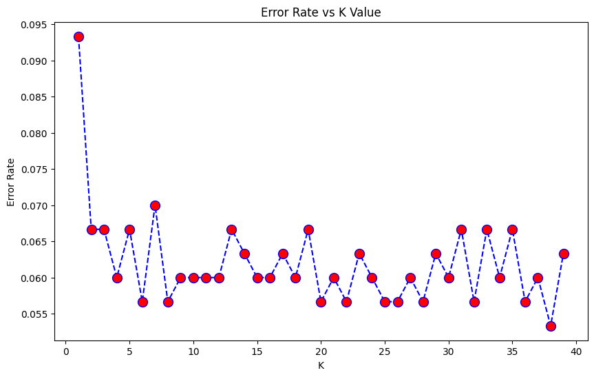
In order to find the best k value it's possible to loop on a range of values and use the loop index to train and predict the model with different k values.
By comparing the error rate it's possible to find the best k value.

error_rate = []

for i in range(1,40):
    knn = KNeighborsClassifier(n_neighbors=i)
    knn.fit(X_train, y_train)
    
    p_i = knn.predict(X_test)
    error_rate.append(
        # average error rate, it's the mean of predicted values that are different from the real values
        np.mean(p_i != y_test)
    )

Plotting the error rate makes easier to find the best k value:

plt.figure(figsize=(10,6))
plt.plot(range(1,40), error_rate, color='blue', linestyle='dashed', marker='o', markerfacecolor='red', markersize=10)
plt.title('Error Rate vs K Value')
plt.xlabel('K')
plt.ylabel('Error Rate')

Finalizing Model

model = KNeighborsClassifier(
    # best key value found in previous step
    n_neighbors=17
)

model.fit(X_train, y_train)

p = model.predict(X_test)

print(confusion_matrix(y_test, p))
print(classification_report(y_test, p))

Results in:

[[141  13]
 [  6 140]]
              precision    recall  f1-score   support

           0       0.96      0.92      0.94       154
           1       0.92      0.96      0.94       146

    accuracy                           0.94       300
   macro avg       0.94      0.94      0.94       300
weighted avg       0.94      0.94      0.94       300