Machine Learning Udemy Bootcamp 06 - Geographical Plotting

Geographical plotting is usually challenging to due the various formats the data can come in.
Plotly is natively able to work with geographical plotting but also matplotlib has a basemap extension.

Choropleth Maps

Choropleth maps provide an easy way to visualize how a variable varies across a geographic area or show the level of variability within a region.

import chart_studio.plotly as py
import plotly.graph_objects as go
from plotly.offline import download_plotlyjs, init_notebook_mode, plot, iplot
import pandas as pd

init_notebook_mode(connected=True)

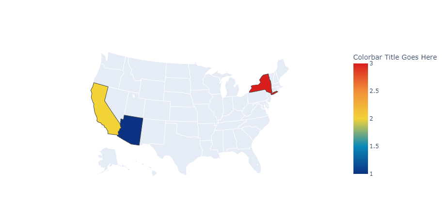
USA

data = dict(
    type='choropleth',
    # states to consider
    locations=['AZ', 'CA', 'NY'],
    # mapping type
    locationmode='USA-states',
    colorscale='Portland',
    # text title of states hover effect
    text=['text1', 'text2', 'text3'],
    z=[1.0, 2.0, 3.0],
    colorbar={
        # title of colorbar
        'title': 'Colorbar Title Goes Here'
    }
)

layout = dict(
    geo={'scope': 'usa'}
)

choromap = go.Figure(data=[data], layout=layout)
iplot(choromap)

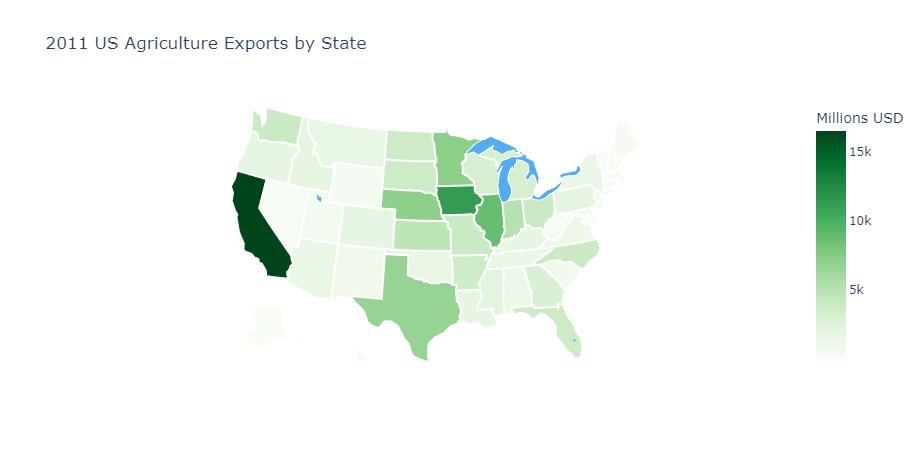
data = dict(
    type='choropleth',
    locations=df['code'],
    locationmode='USA-states',
    colorscale='Greens',
    text=df['text'],
    z=df['total exports'],
    marker=dict(
        line=dict(
            color='rgb(255, 255, 255)',
            width=2
        )
    ),
    colorbar={'title': 'Millions USD'}
)

layout = dict(
    title='2011 US Agriculture Exports by State',
    geo=dict(
        scope='usa',
        showlakes=True,
        lakecolor='rgb(85, 173, 240)'
    )
)

choromap2 = go.Figure(data=[data], layout=layout)
iplot(choromap2)

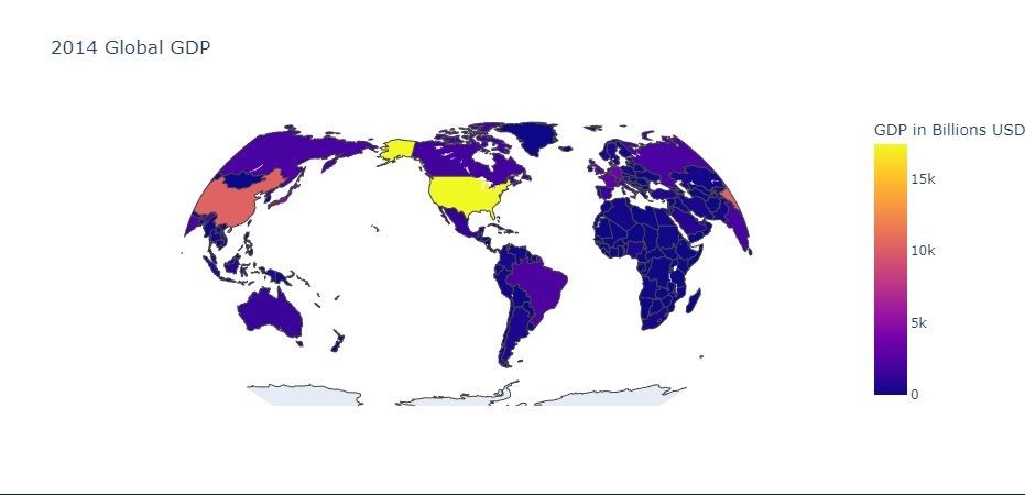
WORLD

df = pd.read_csv('2014_World_GDP')

data = dict(
    type='choropleth',
    locations=df['CODE'],
    z=df['GDP (BILLIONS)'],
    text=df['COUNTRY'],
    colorbar={'title': 'GDP in Billions USD'}
)

layout = dict(
    title='2014 Global GDP',
    geo=dict(
        showframe=False,
        projection={'type': 'natural earth'}
    )
)

choromap3 = go.Figure(data=[data], layout=layout)
iplot(choromap3)